Writing an experiment definition

The purpose of this script is to introduce Signals and guide the reader towards programming in a less procedural way. After reading this you should will be able to create the experiments you want in Signals, using the Signals Experiment Framework. The guide may appear slow at first but sticking with it will greatly reduce the number of errors you will encounter while making your first experiment.

Contents

Introduction

The live script that accompanies this document can be found in signals/docs/turorials/using_signals.m. This script allows you to run the blocks of code shown here and plot the values of signals live. To run a block of code, click on the section of interest and press Ctrl + Enter.

For the purposes of demonstration we can create signals using the sig.test.create function, however in you expDef you can only create new signals based on the function's inputs. More on this later.

function expDefFn(t, events, parameters, vs, inputs, outputs, audio)

Example expDefs can be found in signals/docs/examples.

The bracketed numbers throughout this script correspond to notes at the bottom of the file. The notes provide extra details about Signals. Please report any errors as GitHub issues. Thanks!

What are signals?

When writing an experiment definition (expDef), it's useful to think of signals as nodes in a network, where each node holds a value that is the result of passing its inputs through a function. This network is 'reactive' in that whenever a node's input values change, the node recalculates its own value. In this way changes propergate through the network asynchronously.

The above node graph would be the result of writing the following:

t = sig.test.create; % returns a signal
phi = 2*pi*3*t; % a new signal, phi, that defines phase over time, t

Imagine the signal t was a clock signal whose value was a timestamp that constantly updated. The signal phi then updates it's value every time t updates. In this way you can express relationships between variables in an easy to read, mathematical way. One of these variables happens to be time, which means you can define how variables change over time. In the above example we have defined a temporal fequency in Hz (the value of t in your expDef is in seconds from experiment start). This can then be applied to a visual stimulus property, as shown in the example expDef driftingGrating.m.

Relationships between signals

Let's start to build a reactive network. Most of MATLAB's elementary operators work with signals in the way you would expect, as demonstrated below. You may type ctrl + enter to run this entire secion at once...

x = sig.test.sequence(-50:1:50, 0.05); % Create a sequence
a = 5; b = 2; c = 8; % Some constants to use in our equation
y = a*x^2 + b*x + c; % Define a quadratic relationship between x and y

% Let's call a little function that will show the relationship between our
% two signals.  The plot updates each time the two input Signals update:
ax = sig.test.plot(x,y,'b-');
xlim(ax, [-50 50]);

Mathematical expressions

Signals allows a good degree of clarity in defining methematical equations, particularly those where time is a direct or indirect variable

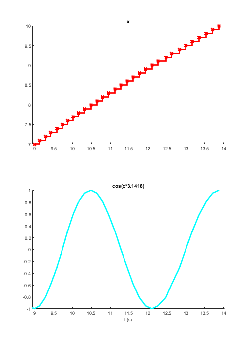
Example 1: cos(x * pi)

x = sig.test.sequence(0:0.1:10, 0.05); % Create a sequence
y = cos(x * pi);
sig.test.timeplot(x, y, 'mode', [0 2]); % Plot each variable against time

Example 2: x -> degrees

Let's imagine you needed a Signal that showed the angle of its input between 0 and 360 degrees:

x = sig.test.sequence(1:4:1080, 0.005); % Create a sequence
y = iff(x > 360, x - 360*floor(x/360), x); % More about conditionals later

sig.test.plot(x, y, 'b-');
xlim([0 1080]); ylim([0 360])

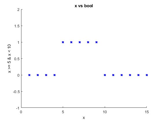
Logical operations

Note that the short circuit operators && and are not implemented in Signals, always use & and | instead.

x = sig.test.sequence(1:15, 0.2); % Create a sequence
bool = x >= 5 & x < 10;

ax = sig.test.plot(x, bool, 'bx');
xlim(ax, [0 15]), ylim(ax, [-1 2])

mod, floor, ceil

A simple example of using mod and floor natively with Signals:

x = sig.test.sequence(1:15, 0.2); % Create a sequence

even = mod(floor(x), 2) == 0;
odd = ~even;

sig.test.timeplot(x, even, odd, 'tWin', 1);

Arrays

You can create numerical arrays and matricies with Signals in an intuitive way. NB : Whenever you perform an operation on one or more Signal objects, always expect a new Signal object to be returned. In the below example we create a 1x3 vector Signal, X, which is not an array of Signals but rather a Signal that represents a numrical array.

x = sig.test.sequence(1:5, 0.5); % Create a sequence
X = [x 2*x 3]; % Create an array from signal x
X_sz = size(X); % Reports the size of object's underlying value

NB: Cell array syntax is not supported in Signals, that is the following won't produce a signal:

X = {x x};
class(X)

   ans =

       'cell'

Although Signals can technically hold cell arrays as their values, it's best to avoid using them in your experiments.

Matrix arithmatic

Xt = X'; % X transpose
Y = Xt.^3 ./ 2;

Complicated expressions

Below are some examples of more complex mathematical expressions that can be defined in Signals.

Example 1: Upper bound

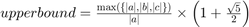
[a, b, c] = sig.test.create('names', {'a','b','c'});

upperBound = max([abs(a), abs(b), abs(c)]) / abs(a) * (1 + sqrt(5))/2;
disp(upperBound.Name)

max([|a| |b| |c|])/|a|*3.2361/2

Example 2: Gabor

Let's reproduce the equation for generating a Gabor patch, i.e convolving a sinusoid with a 2D Gaussian function:

Where:

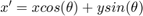
% Create some input signals for this demonstration.  xx and yy are vectors
% of the x and y coordinates of the Gabor, where (0,0) is the centre of the
% Gabor patch
[xx, yy, theta, sigma, lambda, phi] = sig.test.create();

% Create a 2-D grid coordinates based on the coordinates contained in
% vectors xx and yy
[X, Y] = xx.mapn(yy, @meshgrid);

% Calculate the rotated x and y coordinates for the Gabor filter.  The
% rotated coordinates allow us to define an elliptical window rotated by
% theta(1)
Xe = X.*cos(theta(1)) + Y.*sin(theta(1));
Ye = Y.*cos(theta(1)) - X.*sin(theta(1));
% And the rotated coordinates for the grating
Xc = X.*cos(theta(2) - pi/2) + Y.*sin(theta(2) - pi/2);

% Define our Gaussian function
gauss = exp(-Xe.^2./(2*sigma(1)^2) + -Ye.^2./(2*sigma(2)^2));
% The grating function scaled by the wavelegth and translated by the phase
grate = cos( 2*pi*Xc./lambda + phi );
G = gauss.*grate; % Convolve the two functions

Every signal has a Name property that you can print or set. This is useful for plotting and visualizing signals. Below we rename some of our signals to Greek letters then print our Gabor signal name:

% Rename a few of our signals for display purposes
theta.Name = char(hex2dec('03bb')); % Orientation
sigma.Name = char(hex2dec('03B8')); % Standard deviation of Gaussian envelope
lambda.Name = char(hex2dec('03C3'));% Wavelength
phi.Name = char(hex2dec('03C6')); % Phase offset
Xe.Name = 'x'''; Ye.Name = 'y'''; % Rename to X' and Y'
X.Name = 'x'; Y.Name = 'y'; % Rename to x and y

% And print their names to the command window
fprintf([...
  'Gaussian equation: %s\n',...
  'Grating equation: %s\n',...
  'Convolved: %s\n'],...
  gauss.Name, grate.Name, G.Name)

Gaussian equation: exp((-x'.^2./2*θ(1)^2 + -y'.^2./2*θ(2)^2))
Grating equation: cos((6.2832*(x.*cos((λ(2) - 1.5708)) + y.*sin((λ(2) - 1.5708)))./σ + φ))
Convolved: exp((-x'.^2./2*θ(1)^2 + -y'.^2./2*θ(2)^2)).*cos((6.2832*(x.*cos((λ(2) - 1.5708)) + y.*sin((λ(2) - 1.5708)))./σ + φ))

The above code is simply a demonstration of how to express relationships mathematically in Signals. In the next tutorial we will look at creating stimuli in Signals. Spoiler: there's a function that creates a Gabor for you.

To live-plot a couple of interesting mathematical functions using Signals, see the end of this guide.

A note about Signals variables

Signals are objects that constantly update their values each time the Signals they depend on update. When you do an operation on a signal (e.g. x * 2) a new Signal object is created. This can be assigned to a variable (e.g. y = x * 2, however clearing or overwriting that variable does not affect the underlying Signal. The original object stays around until its inputs or the network are deleted. This is important to think about when writing expDefs. Think of variables as temporary labels for each object which can be moved around at any time without affecting the object they label. Consider the following:

% Create a new input signal and assign it to the variable 'a'
a = sig.test.create();
% Derive a new signal from 'a' and assign it to the variable 'b'
b = abs(a);

% Reassign a value to 'a', e.g. a string.  Think of this as taking a
% sticker that says 'a' off the Signal object and placing it on a string
% instead:
a = "hello"; % assign "hello" to variable 'a'.
% Note that this doesn't affect the Signal object originally assigned to
% 'a', but now if you do something to 'a', you're not working with a Signal
% anymore, but rather a char array:
b = abs(a)

  Undefined function 'abs' for input arguments of type 'string'.

This may seem obvious but important to note as this can be unclear to people not used to this way of programming.

Likewise if you re-define a Signal, any previous Signals will continue using the old values and any future Signals will use the new values, regardless of whether the variable name is the same. Remember that variable names are simply object handles so clearing or reassigning those variable names doesn't necessarily change the underlying object:

% Let's start with a blank slate
clear variables
% Create a new input signal, x, and assign it to the variable 'a'
a = sig.test.create('names', "x");
b = a^2; % Derive a signal ('a^2') and assign it to variable 'b'
c = b + 2; % Derive a new signal ('a^2 + 2') and assign it to variable 'c'
b = a*3; % A new Signal object ('a*3') is assigned to the variable 'b'
d = b + 2; % A new Signal object ('a*3 + 2') is assigned to the variable 'd'

The key here is that d has the value a*3 + 2 and not a^2 + 2, even though the variable b was at one point a^2. Counting each mathematical value in the above code block (i.e. mathematical variables and constants), how many nodes are in our network? The answer is 9 (see note 2).

Variables are like labels, if you reassign them they are no longer pointing to the same object.

Looking at the name of your Signals may help you better understand what they are

y = abs(a);
disp(['y = ' y.Name])

y = y^2;
disp(['y = ' y.Name])

z = [y y];
disp(['z = ' z.Name])

y = |a|
y = |a|^2
z = [|a|^2 |a|^2]

It's fine to break long lines into multiple shorter lines by re-assigning to the same variable:

b = a * 2 * pi;
b = abs(b);
disp(b.Name)

b = |a*2*3.1416|

Signals only update when all their inputs have have values

As you may have noticed, signals can be derived from any number of other signals, as well as by constants(3). Mathematically, Signals can be viewed as variables which, any time they take a new value, cause any dependent equations to be re-evaluated.

This leads us to one of the most important things to consider when writing an expDef: Signals can only update if all (or enough) of their inputs have values.

At the beginning of an Experiment your expDef function is called and all your signals are wired up. Until the experiment starts however, none of these signals have any value. Each signal can only update its value when its inputs have updates and the time that this happens depends on how you wire your network.

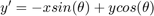
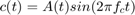
In the below example we have signals x, a, b, and c. From these, we derive a new signal and assign it to 'y'. If x updates, y won't because the expression is still incomplete, we don't have values for a, b, or c. Likewise if b updates, y will remain unchanged and any signals derived from y will likewise not update. The signal y can only have a value once all the input signals have a value. When all inputs have values, a change to any of the inputs will cause y to be revaluated using the most recent value of all the inputs.

% Here we create four signals that each update in staggered fashion:
x = sig.test.sequence(1:5, 1, 'delay', 1); % Update once per second after a second
a = sig.test.sequence(1, 1, 'name', 'a', 'delay', 2); % Update after 2 seconds
b = sig.test.sequence(1, 1, 'name', 'b', 'delay', 3); % Update after 3 seconds
c = sig.test.sequence(1, 1, 'name', 'c', 'delay', 4);  % Update after 4 seconds

y = a*x^2 + b*x + c;

sig.test.timeplot(x, a, b, c, y);

As you can see from the above plot, the signal 'y' does not update until all its input signals have values. Once all of its inputs have a value whenever any of them updates a new value is calculated using the most recent values of each input.

Conditional statements

iff

Above we saw how logical operations work with Signals. These can also be used in conditional statements that alter the value or operation on a given Signal. Using an if/else statement won't work in your expDef. To construct something similar to an if/else statement, we can use the iff method:

% Create a signal whose values go from 1 - 200
x = sig.test.sequence(1:2:200, 0.05);
% if x is greater than 100, y = 100, otherwise y = x
y = iff(x > 100, 100, x);

% Plot the results
ax = sig.test.plot(x, y, 'k-');
ax.XLim = [0 200]; ax.YLim = [0 200];

Note that with iff any and all values can be signals. Also note that iff is also a Rigbox function that works outside of signals:

x = 'd';
added = iff(ischar(x), @() [x x], @() x + x)

cond

In order to construct if/elseif statements we use the cond method, where the input arguments are predicate-value pairs, for example:

y = cond( ...
  x < 5, a, ... % If x < 5, y = a
  x > 10, b); % elseif x > 10, y = b

As with all Signals, the condition statement is re-evaluated when any of its inputs update. Any input may be a Signal or otherwise, and if no predicate evaluates as true then the resulting Signal does not update.

Likewise, the condition statement will terminate if any of the source Signals of a particular pred-value pair do not yet have values. Also, in the same way as a traditional if-elseif statement, each predicate is only evaluated so long as the previous one was false. For this reason, the order of pred-value pairs is particularly important. Below we use true as the last predicate to ensure that the resulting Signal always has a value.

y = cond(...
  x > 0 & x < 5, a, ... % if x between 0 and 5, y = a
  x > 5, b, ... % elseif x is greater than 5, y = b
  true, c); % else y = c

Indexing

Indexing into a Signal

Signals can be indexed as expected with brackets and the colon operator.

A = sig.test.create;
a = A(2); % index second element of A
B = A(5:end); % index elements 5 to array end

Indexing with a Signal

Another Signal may be used to index another Signal. In the below example we derive a signal indexes the value of A with the value of i. The resulting signal will update whenever i or A update, so long as both of them have a value.

i = sig.test.create; % Define a new Signal
a = A(i);

If the value of A has a length less than the value of i, an 'index out of bounds' error will be thrown, just like with normal arrays. One solution to this would be to use a conditional signal like the one in the previous section to deal with such cases:

i = iff(i > numel(A), numel(A), i);
a = A(i);

selectFrom

The selectFrom method allows for indexing from a list of Signals whose values may be of different types. In some ways this is comparable to indexing into a cell array:

y = i.selectFrom(A, B, C); % when i == 1, y = A, etc.

NB: When the index is out of bounds the Signal simply doesn't update. This could also be used to e.g. map a choice signal to a bunch of outcome signals.

indexOfFirst

The indexOfFirst method returns a Signal with the index of the first true predicate in a list of Signals. This has a similar functionality to find(arr, 1, 'first'):

idx = indexOfFirst(A > 5, B < 1, C == 5); % Better examples welcome!

NB If not all input signals have values, or none of them are true (i.e. non-zero) then the value idx will equal the number of inputs + 1. This is a rare exception to the rule that signals don't update unless all their inputs have a values. The below example will produce a signal that will only update with a valid index:

idx = indexOfFirst(x, y, z);
% Keep when value is less than or equal to number of inputs (i.e. 3)
idx = idx.keepWhen(idx < 4);

map

Not all MATLAB functions work natively with Signals. For example, the function ischar does not play nicely with Signal objects:

A = sig.test.create; % Create an new signal
B = ischar(A);
class(B) % Note that B is not a Signal object but a boolean.

In the above example, MATLAB is testing the object itself, rather than the value of A (see note 4). For this reason B isn't a Signal object and will never be true, even is the value of signal A is a char. The solution to this problem is to use the map method.

map creates a new signal that calls an arbitraty function with the value of its input. This new signal's value is the output of the function you give it.

B = A.map(@ischar);
class(B) % Returns a Signal object

In the above example whenever signal A updates with a new value, its value is passed (or 'mapped') to the function ischar and the output (a boolean) becomes the value of signal B. This means that B will update its value whenever A updates. As usual, while A doesn't have a value, ischar is never called.

The @ symbol is MATLAB's syntax for a function handle. Instead of calling the function, you simply point to the function as if it is a variable. For more information, see the MATLAB documentation on creating function handles.

In the below example we create a signal that can checks whether its input is a char and if so, converts it to a number:

B = iff(A.map(@ischar), str2num(A), A);

Why use can we write str2num(A) and not ischar(A)? You can see which methods work natively with Signals by looking at the following list:

methods('sig.Signal') % All methods of the class sig.Signal

   Methods for class sig.Signal:

   Signal        buffer        delta         floor         keepWhen      map2          mod           onValue       rot90         sin           times
   abs           bufferUpTo    eq            ge            lag           mapn          mpower        or            round         skipRepeats   to
   all           colon         erf           gt            le            max           mrdivide      output        scan          sqrt          transpose
   and           cond          exp           horzcat       log           merge         mtimes        plus          selectFrom    str2num       uminus
   any           cos           fliplr        identity      lt            min           ne            power         setTrigger    strcmp        vertcat
   at            delay         flipud        indexOfFirst  map           minus         not           rdivide       sign          sum

   Methods of sig.Signal inherited from handle.

As you can see str2num is in the list but ischar is not. If in doubt, map will always work, it just looks a little uglier:

B = iff(A.map(@ischar), A.map(@str2num), A);

Another important thing to note is that operators like '==' and '*' are just convenient ways of calling normal functions (5). They actually correspond to the functions eq and times. Most of the time you can use either form but on occasion it's clearer to use one over the other.

B = iff(A.map(@ischar), strcmp(A, '10'), A == 10)
B = iff(A.map(@ischar), strcmp(A, '10'), eq(A, 10)) % These are equivalent

The functions you call using map can be any function include your own non-builtin functions (although they need to be on the MATLAB search path). You can also define local functions in your expDef and map values with those. The functions used by map don't need to deal with Signal objects as they only get called with a signal's value.

What if your function expects single but your input signal's value is a double? Simply typecast it with map!

B = A.map(@single).map(@myfunc);

The value of A is called on single and its output is then called on myfunc. You'll notice that many Signals methods can be chained in this way, which is convient for writing one-liners. If your line becomes too long or difficult to read you can also split it across a number of lines:

B = A.map(@single);
B = B.map(@myfunc);

Anonymous functions

Sometimes your Signal must be in a different positional argument. For this we simply create an anonymous function and use that. See the MATLAB doumentation for more information on how to use these.

delta = A.map(@(A) diff(A,1,2)); % Take 1st order difference over 2nd dimension
a = A.map(@(A) sum(A,2)); % Take sum over 2nd dimension

You may have noticed that our other example can be written using an anonymous function as a wrapper so that map is called just once:

B = A.map(@(v) myfunc(single(v)));

Any of these variants will work just fine and there is no real atvantage to which one you choose, however if you need to access the intemediate value (i.e. single(v), it is better to use the former example.

Example 2: a complex counter

In the following example we have a signal, responseType, that may be an element of [-1 0 1]. A response type of 0 means the trial timed out before the subject gave a response. Let's say we want to count the number of times in a row a trial timeout occurs:

% First we store the responseType values for up to the last 1000 trials
timeOuts = responseType.bufferUpTo(1000);
% Then count the number of recent timeouts that occured in a row using an
% anonymous function that works on this array with find and sum:
timeOutCount = timeOuts.map(@(x) sum(x(find([1 x~=0],1,'last'):end) == 0));

Sampling with map

Map is particularly handy for 'sampling' functions, that is, for generating a new index, value, or whatever, each time an event occurs. Below we derive a signal, 'side', that each time 'newTrial' updates takes a new value from [-1 1]. Note that the anonymous function discards the value of 'newTrial'. We're only using it as a way to trigger the evaluation of this function.

newTrial = sig.test.create;
side = newTrial.map(@(~) sign(rand-0.5));

at

The method at will sample the value of a Signal each time another Signal updates. What's more, the Signal that updates must evaluate to true:

x = sig.test.sequence(1:1:100, 0.15); % An linear function
y = sig.test.sequence(sin(1:.1:20), 0.1, 'name', 'y'); % A sine wave
z = x.at(y > .5); % sample the values of x when the values of y > 0.5

sig.test.timeplot(x, y, z, 'mode', [2,2,1], 'tWin', 20); % plot over 20 secs

It's very important to remember that the new signal will only update when the second input updates and is true (so long as the first input has a value to sample). For the value to be true, it must not be equal to 0. In other words, y = x.at(updatedAndNonZero). As you can see 'z' keeps updating each time 'y' updates, even when 'x' stops updating (c.f. keepWhen method below).

Below is an example of how to implement downsampling, or 'throttling', of a signal:

t = sig.test.sequence(0:0.1:30, 0.1, 'name', 't');
x = sin(t);

% Sample at 1Hz, i.e. whenever t is a multiple of 1
sampler = skipRepeats(floor(t)).then(true);
throttled = x.at(sampler);

sig.test.timeplot(t, x, throttled, 'mode', [2 2 1], 'tWin', 30);

then

There is another method called then which works the same way as at, but with the inputs in a reverse order. This is simply to make things more self-documenting.

updatedAndTrue = y.at(updated);
updatedAndTrue = updated.then(y); % These two lines are equivalent

Mapping constants

Sometimes you want to derive a Signal whose value is always constant but nevertheless updates depending on another Signal, thus acting as a trigger for something. This can be achieved by using a constant value instead of a function in map. For example below we produce a signal that is always mapped to true and updates whenever its dependent value updates.

seq = repmat(-2:2, 1, 5);
x = sig.test.sequence(seq, 0.2); % Create a sequence
y = x.at(x); % Zero values are ignored
updated = x.map(true); % Updates to true each time x updates
z = x.at(updated); % All values map to true

ax = sig.test.timeplot(x, y, z, 'mode', [0,1,1]);

The above example is simply to demonstrate that you can map a value to 'true' when we care about the 'when' of a signal than the 'what'. In the above code x and z do the same thing, but would be useful when you want to sampling one signal each time differnt signal updates, e.g.

updated = y.map(true);
z = x.at(updated);

Note that if the input arg is a value rather than a function handle, it is truely constant, even if it's the output of a function:

c = x.map(rand); % use constant value of rand each times x updates
rnd = x.map(@(~)rand); % call rand each time x updates

The tilda here means that the value of Signal x is ignored, instead of being assigned to a temporary variable or being mapped into the functon rand, thus rand is called with no arguments.

keepWhen

Another method for filtering signals is keepWhen. This will keep the value of one signal so long as another signal evaluates true (i.e. is non-zero).

x = sig.test.sequence(1:15, 0.25); % Create a sequence
isEven = mod(floor(x), 2) == 0; % True when x is an even number
y = x.keepWhen(isEven); % Sample x when x is even

ax = sig.test.timeplot(x, y, 'mode', 1);

What's the difference between keepWhen and at / then? These two methods essentially do that same thing, however the result of keepWhen will update each time its first input updates, so long as its second input is non-zero.

x = sig.test.sequence(1:1:100, 0.25); % A linear function updating every 1/4 second
y = sig.test.sequence(sin(1:.1:20), 0.1, 'name', 'y'); % A sine wave updating every 100ms

% z = x.at(y > .5); % z stops when y stops updating
z = x.keepWhen(y > .5); % z stops when x stops updating
sig.test.timeplot(x, y, z, 'mode', [2,2,1], 'tWin', 20);

Try playing with the update times and using at vs keepWhen.

NB: In version 1.3, keepWhen can be used in the same way as filter. The below lines are equivalent.

y = x.keepWhen(x > 0);
y = x.keepWhen('> 0');

filter

NB: This method will be introduced in version 1.3. The filter method filters the values of the input based a function. The function should except a single input and output a logical value. By default values that evaluate true are kept:

x = sig.test.sequence(sin(1:.1:10), 0.2);
y = x.filter(@(x) x > 0);

sig.test.timeplot(x, y, 'mode', [2 1], 'tWin', 20);

The function handle may be a char:

y = x.filter('isinteger');
y = x.filter(@isinteger); % These two are equivalent

For simple logical operators the lefthand side can be omitted:

y = x.filter('~= 0'); % Keep non-zero values
y = x.filter(@(x) x ~= 0);
y = x.filter('x~=0');
y = x.filter(@identity); % These four are equivalent

NB The same behaviour can be achieved with keepWhen. The below lines are equivalent also:

y = x.keepWhen(x ~= 0);
y = x.keepWhen('~=0');

An optional input argument allows you to explicitly set the criterion, which is true by default:

y = x.filter(@isnan, false); % Keep non-empty values
y = x.filter(@(x) ~isnan(x)); % These two are equivalent
y = x.filter('~isnan(x)'); % A char can be used as long as you use 'x'

The criterion may also be a signal, allowing you to keep either the passed or failed values on the fly. In the below example the positive values are kept only on odd trials:

keepTrue = events.trialNum.mod(2); % False on even trials
y = x.filter('>0', keepTrue);

Note that a non-signals filter function is also available in Rigbox:

% fun.partial returns a function with the first argument pre-set
filter = fun.partial(@fun.filter, @isnan); % equivalent to @(x)fun.filter(@isnan,x)
[passed, failed] = x.mapn(filter);

skipRepeats

skipRepeats creates a signal that only updates when its input updates with an unique value. That is, when its input updates with a value that is different to the previous one. It is important to realize that signals can repeatedly update with the same value, and each time a signal updates it can cause other signals to update depending on how you define them. Below is an example of skipRepeats:

seq = [0 0 2 2 0 0 -2 -2 0 0 0];
x = sig.test.sequence(seq, 0.45);
y = skipRepeats(x);

sig.test.timeplot(x, y);

A signal that updates only once

In this next example we show how to define a signal that updates once and only once. Remember that signals generally update whenever any of their inputs update. Sometimes you want to use a value such as a user defined parameter to calculate something, but you don't want it to change at all.

x = sig.test.sequence(0:9, 0.5);
y = x.map(true).skipRepeats.then(x);

sig.test.timeplot(x, y, 'mode', 1);

Here is a similar example: update once and only once, when x is zero

x = sig.test.sequence(-4:4, 0.5);
y = x.keepWhen(x == 0).skipRepeats;

sig.test.timeplot(x, y, 'mode', 1);

A note about syntax

When we type something like A.map(pi) we are actually calling the method map on the object A. A method is another word for a function associated with an object. Signals are objects, and so far we've looked at various methods (i.e. functions) that work with them. In MATLAB there are two ways of calling a method on an object, one is the traditional way e.g. func(obj) and the other is the 'dot syntax' way: obj.func(). These are the same, and you can use them interchangeably so long as 'obj' is a Signal (and not something else, like a double or logical). Below are pairs of lines that are equivalent:

S = sig.test.create; % create a Signal object

S = S.map(pi); % Map values of S -> pi, e.g. when S updates, return pi
S = map(S, pi);

S = S.then(true); % When S updates and is true, return true
S = then(S, true);

This dot syntax is very useful for chaining together methods in a way that is terse and readable. Below we chain together functions to define y as the sum of the absolute changes in x. This is a core

x = sig.test.create('names', "x");
y = x.delta.abs.skipRepeats.scan(@plus);

disp(['y = ', y.Name]) % y = (*|?x|).scan(@plus)

These chains can be spread over multiple lines using elipses:

y = x.delta. ...      % Take the change in x
    abs. ...          % Make it absolute
    filter('>10'). ...% Keep only values greater than 10
    skipRepeats. ...  % Skip if the same as the last value
    scan(@plus). ...  % Add it to our accumulated value
    map(@string). ... % Convert to string
    buffer(10);       % Store the last 10 strings in an array

mapn

mapn takes any number of inputs where the last argument is the function that the other arguments are mapped to. The arguments may be any combination of signals and normal data types. It's important to note that the below 'dot notation' only works if the first input is a Signal, otherwise you must use the traditional syntax e.g. mapn(5, A, @f)

B = A.mapn(n, 1, @repmat); % repmat(A,n,1)

NB: map will only assign the first output argument of the function to the resulting Signal. Mapping to a variable number of output Signals is only possible with mapn:

a = sig.test.create; % if a = rand(1,1,3,1,2)
[b, n] = a.mapn(@shiftdim); % b is 3-by-1-by-2 and n is 2.
c = b.mapn(-n, @shiftdim);  % c == a.
d = a.mapn(3, @shiftdim);   % d is 1-by-2-by-1-by-1-by-3.

map2

If you have exactly two inputs to a function you can also used map2. This method behaves identically to mapn but can apply a function to only two inputs. Also map2 cannot create more than one resulting signal.

% Load an image from a directory of images with the name pattern imgN.mat:
imgArr = imgIdx.map2(imgDir, ...
  @(num,dir)loadVar(fullfile(dir, ['img', num2str(num), '.mat']), 'img'));

scan

scan is a very powerful method that allows one to map a signal's current value and its previous value through a function. This allows one to define signals that have some sort of history to them. This is similar to the fold or reduce functions found in other functional programming applications (see note 6).

Below we take the value of x and return a value that is the accumulation of x by using scan with the function plus. The third argument to scan here is the initial, or 'seed', value. Because the seed is zero, the first time x takes a value, scan maps zero and the value of x respectively to the plus function and assigns the output to Signal y. The second time x updates, scan maps the current value of y - our accumulated value - and the new value of x to the plus function.

x = sig.test.sequence(ones(1:10), 0.5);
y = x.scan(@plus, 0); % y = plus(y, x), or y = y + x

sig.test.timeplot(x, y);

The seed value may be a signal

As with other Signals methods, any of the inputs except the function handle may be a Signal. This is particularly useful as the seed value can act as a reset of the accumulator as demonstrated below. The seed must have a value before the signal will update.

x = sig.test.sequence(1:10, 0.5);
seed = sig.test.sequence([0 0], 2.5, 'name', 'seed');
y = x.scan(@plus, seed);

sig.test.timeplot(x, y, seed, 'mode', [0 0 1]);

Growing an array with scan

You can grow arrays with scan by using the vertcat or horzcat functions. The accumulated/seed value is always the first argument to the function, however, you can of course assign them to temporary variables beforehand as below.

x = sig.test.sequence('olleh', 1);
f = @(acc,itm) [itm acc]; % Prepend char to array
y = x.scan(f, '!');

sig.test.timeplot(x, y); % Plot values
h = output(y); % Print value to command prompt

Below, each time the Signal 'correct' takes a new, non-zero value, the Signal 'trialSide' updates and scan will call the function horzcat with the values of 'hist' and 'trialSide' like so: horzcat(hist, trialSide), which is syntactically equivalent to [hist trialSide]:

hist = trialSide.at(correct).scan(@horzcat);

NB: that is can also be acheived using the bufferUpTo method, however scan gives one the ability to reset the history (i.e. clear the buffer) at any time.

Example: finding the max with scan

In this example we use scan to find the maximum value in a signal's history. The logic is simple: each time signal 'x' updates we compare our previous max value with the new one and save whichever is bigger.

Let x be an amplitude modulated signal defined as:

f_c = 8; % Carrier frequency in Hz
t = 0:1/1000:0.5; % Determine time values at 1000 Hz sampling rate
A = t % Information signal (linear function)

% Define AM signal
AM = A.*sin(2*pi*f_c*t);
x = sig.test.sequence(AM, 0.1);

peak = x.scan(@max, -Inf).skipRepeats();

sig.test.timeplot(x, peak, 'mode', [2, 1], 'tWin', 60);

Example: Keep the unique values of a signal

x = sig.test.sequence(randi(10,1,50), 1);
xU = x.scan(@union, []);
h=output(xU);

Example: Keep track of which values in a set have not yet occurred

x = sig.test.sequence(randi(10,1,25), 1);
set = [1 2 4 7];
remaining = x.scan(@setdiff, set);
allOccurred = remaining.map(@numel) == 0;

plotArgs = {'tWin', 15, 'mode', [0 1 1]};
ax = sig.test.timeplot(x, remaining, allOccurred, plotArgs{:});
ax(2).YLim = [-Inf max(set)+1];
h = output(remaining);

Introducing extra parameters

Some functions require any number of extra inputs. A function can be called with these extra parameters by defining them after the 'Pars' name argument. All arguments after the 'Pars' input are treated as extra parameters to map to the function when either the input or seed Signals update. Parameters can be normal values, signals or a mixture of the two. Below we use the scan function to build a character array with strjoin...

x = sig.test.sequence(["1" "12" "18" "5" "8"], 1);
seed = sig.test.sequence("0", 1, 'delay', 0); % Initialize seed with value
f = @(acc,itm,delim) join([acc, itm], delim); % Prepend char to array
y = x.scan(f, seed, 'pars', ' + '); % Pars may be signals or any other data type
h = y.output();

When pars take new values, accumulator function is not called!

Unlike most other Signals, parameters Signals can take new values without causing the function to be called. Below we define a Signal, p, into which we can post the delimiter for the function strjoin.

x = sig.test.sequence(randi(10,1,5), 1); % Some random numbers from 1-10
p = sig.test.sequence('+-', 1, 'name', 'op'); % Some operators
init = '0'; % The seed value
f = @(acc,itm,delim) strjoin({acc, num2str(itm)}, delim); % Prepend char to array
y = x.scan(f, init, 'pars', p); % Pars may be signals or any other data type

h = y.output(); % Output to the command window
sig.test.timeplot(x, p, y); % Plot values

Plot output

Command output

   0+1
   0+1-10
   0+1-10-8
   0+1-10-8-8

Note that y can not update until all its inputs have values (i.e. we don't see a value until p updates).

Stateful data structures

So far we've looked at using scan to accumulate and reduce arrays, however scan is perhaps most useful when applied to structs. Scan can be used to maintain a data structure which holds information about the current state of things. For this to work, the seed value should be a struct.

In the below example from the choiceWorld example expDef we create a signal array of some things we want to track, namely the final position of the stimulus, the trial number, the response ID and the current bias. This is fed into a function called updateTrialData via scan, with the initial value being an empty struct (it could also be a struct with initial values). The output is an updated struct which we can then apply as parameters to the visual stimulus, etc.

% Update performance at response
responseData = vertcat(stimDisplacement, events.trialNum, response, bias);
trialData = responseData.at(response)... % At response time
            .scan(@updateTrialData, struct)... % feed in our response data
            .subscriptable; % mak the output signal subscriptable
% Set trial contrast (chosen when updating performance)
trialContrast = trialData.contrast.at(events.newTrial);
hit = trialData.hit.at(response); % Was it a correct response?

The function as the following signature: function trialData = updateTrialData(trialData,responseData) % Update the performance and pick the next contrast stimDisplacement = responseData(1); response = responseData(3); % bias normalized by trial number: abs(bias) = 0:1 bias = responseData(4)/10; ... % Define response type based on trial condition trialData.hit = response~=3 && stimDisplacement*trialData.trialSide < 0; % Pick next contrast trialData.contrast = randsample(contrasts, 1, true, w); % Pick next side trialData.side = iff(rand <= 0.5, -1, 1); ...

As you can see the output is a struct of with fields such as 'contrast' which we can then use in our expDef. In order to do this we use the subscritable mathod to make sure that we can use subsref on the trialData signal, i.e. contrast = trialData.contrast. If the field you are referencing doesn't exist, your signal simply won't update. If and when your scanning function adds the field, the signal will update with that signal's value.

This sort of stateful data structure is particularly handy for implementing a reinforecement learning algorithm, where at given timesteps information is fed into the scanning function, along with the sate of the previous timestamp, and an updated state is returned.

Scan can call any number of functions at the same time

Scan can call any number of functions each time one of the input Signals updates. Only the functions whose named inputs update will be called. Remember that all functions called by scan have the accumulated value as their first input argument, followed by the input Signal and any parameters following the 'pars' input.

Below is simple example to demonstrate the signature of scan with multiple functions. When x updates, the plus is called with the current value of v and x, and the output is assigned to v. Likewise, when y updates, minus is called with the current value of v and y, and the output is assigned to v. Any number of functions and can be called in this way. The seed value and any parameters added are used in all functions, therefore the seed should have the correct identity value (0 for plus, 1 for times) and the functions should have the same signature, namely acc = f(acc, v, p1,...,pN).

f1 = @plus; % v = plus(v, x)
f2 = @minus; % v = minus(v, y)
f3 = @times; % v = times(v, z)
v = scan(x, f1, y, f2, z, f3, seed);

Now let's look at an example with structs. Below shows how the setEpochTrigger method is actually implemented using scan:

% Get functions for the scanning signal
[initState, tUpdate, xUpdate] = sig.scan.quiescienceWatch;
% Each time period updates, return a default state structure
newState = period.map(initState);
% Update state structure each when t and x signals change
state = scan(t.delta(), tUpdate,... scan time increments
             x.delta(), xUpdate,... scan x deltas
             newState,... initial state on arming trigger
             'pars', threshold); % parameters
state = state.subscriptable(); % allow field subscripting on state

% event signal is derived by monitoring the 'armed' field of state
% for new false values (i.e. when the armed trigger is released).
armed = state.armed;
% Update to true; update only when trigger released
tr = armed.skipRepeats().not().then(true);

Take a look at the functions in sig.scan.quiescienceWatch to get an idea of what's happening when each one is called. Note that tUpdate and xUpdate each have three inputs, even though xUpdate doesn't use the third input, it is always called with the threshold parameter.

By using multiple functions you can compartmentalize your code, where different fields are handled by different functions. The +scan package contains functions that return function handles for use with scan. In the future more of these general-purpose functions will by added.

Example: buffer with scan

The below code shows how something like the buffer method could be inplemented with scan:

buffupto = scan(x, buffering(nSamples), []);
nelem = size(buffupto, 2);
b = buffupto.keepWhen(nelem == nSamples);

function f = buffering(maxSamples)
%SIG.SCAN.BUFFERING Implement buffering with scan
%   Returns a function which grows an array up to the size of
%   'maxSamples'.

f = @buffer;

   function buff = buffer(buff, val)
     if size(buff, 2) == maxSamples
       buff = cat(2, buff(:,2:end), val);
     else
       buff = [buff val];
     end
   end

end

subscriptable

The subscriptable method allows you to derive signals from ones that have structs as their values. Subscriptable signals are referenced just like normal structs. If the field you are subscripting doesn't exist, the resulting signal will simply never update. In the below example we create a couple of signals that update with a struct to demonstrate the behaviour of the subscriptable method.

% Create array of structs which our sequence signal will update with
s = {struct('foo', 1), ...
     struct('foo', 2, 'bar', 'baz'), ...
     struct('foo', 3)};
s = sig.test.sequence(s, 1, 'name', 'subscriptable');

s = s.subscriptable; % Make signal subscriptable
foo = s.foo; % This field changes value from 0 to 1
bar = s.bar; % This field appears after a second
nil = s.nil; % This field isn't here

% Plot our signals against time
sig.test.timeplot(s, foo, bar, nil, 'tWin', 2.5, 'mode', 1);

NB: The subscript referencing happens 'at runtime', i.e. at the time the signal updates. If the subsciptable signal's value is not a struct, an error will be thrown. If your signal is likely to change datatype, consider using keepWhen to filter by datatype before deriving the subscriptable signal:

% Update only when s updates with a value that is a struct
s = s.keepWhen(s.map(@isstruct)).subscriptable()

delta

x = sig.test.sequence(linspace(-1,1,50).^2, 0.1);
y = delta(x);

sig.test.timeplot(x, y, 'mode', 2);

lag

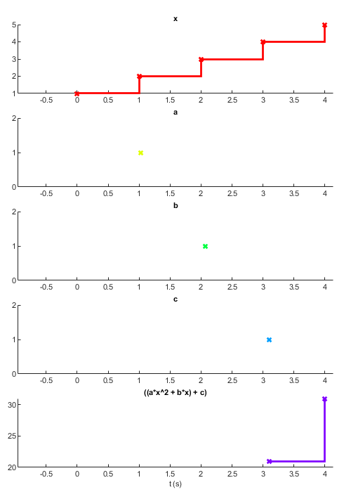
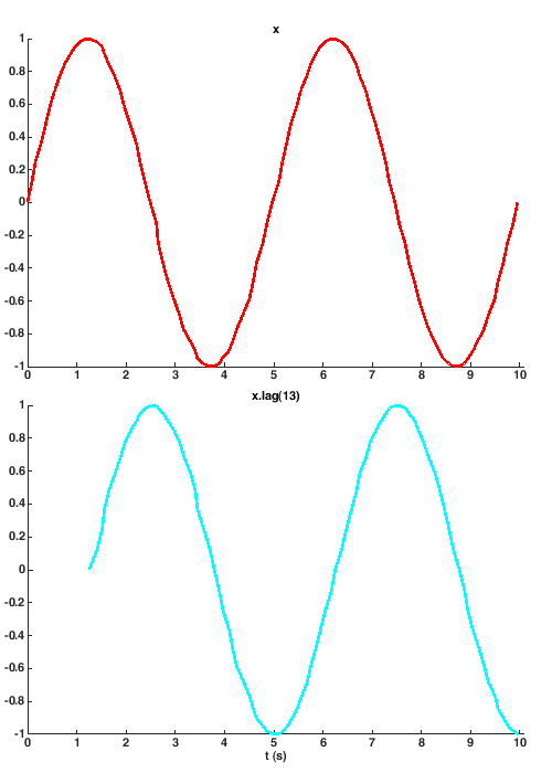
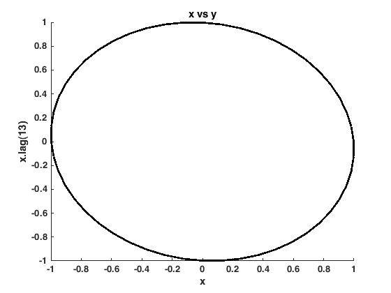
lag delays a signal by a given number of samples. To delay by a given amount of time, use delay. The number of samples you delay by must be a positive whole number or a signal with such a value. The derived signal will only update once the input signal has updated the minimum number of times. That is, given b = a.lag(5), 'b' will get its first value after 'a' has updated five times.

In the below example we define a sine wave signal, then derive a signal that lags by a quarter of a period. Plotting these two against each other results in a circle.

f = 2; % Frequency in Hz
Fs = 100; % Samples per second
t = 0 : 1/Fs : 2/f; % 2 periods

x = sin(2*pi*f*t); % A sine wave
x = sig.test.sequence(x, .1); % Update every 100ms

% Derive a signal that lags by T/4 samples
y = x.lag(round(Fs/(4*f)));

sig.test.timeplot(x, y, 'mode', 2, 'tWin', 10); % Plot vs time
sig.test.plot(x, y, 'k-'); % Plot x vs y

buffer

The buffer method stores the last N values of its input. Each time the dependent signal updates, the new value is appended to an array of previous values. Unlike bufferUpTo, buffer will only update once all the 'buffer slots' have been filled. That is, when the input signal has updated N times.

The number of samples to buffer (N) must be a positive whole number. If N = 0 the buffer signal never updates, if N = 1 then the buffer signal updates with the same value as the input signal (to update with the input signal's previous value, use x.lag(1)). If N = 2 the buffer updates with the last two values, and so on.

x = sig.test.sequence(1:5, 1); % x counts to 5, updating every second
y = x.buffer(3); % Buffer the last three values of x

h = output(y);

    1     2     3

    2     3     4

    3     4     5

NB: Starting version 1.3, the buffer number may be a signal, in which case updates to this signal will not cause the buffer to change, but the next time the signal that's being buffered updates, the buffer array size is adjusted. Remember the buffer signal won't update if the number of previous values < the buffer size, N.

x = sig.test.sequence(1:6, 1); % x counts to 6, updating every second
n = sig.test.sequence([2, 2, 3, 2, 1], 1); % Keep adjusting the buffer size

b = x.buffer(n);
h = output(b); % Print the values of b to the command window

    2     3

    2     3     4

    4     5

    6

The buffer array is always the result of horizontally concatinating the input values. Therefore the size of your input signal's value must remain consistant. You can build an N-D array with the buffer if your input signal's values are vectors or matrices so long as they can be horizontally concatinated. Below we create a matrix by building up the column arrays:

x = sig.test.sequence(1:6, 1); % x counts to 6, updating every second
xT = x.buffer(2).'; % store the last two values transposed to form a 2x1 vector
y = xT.buffer(3); % Buffer the last three values of xT to form a 2x3 matrix

h = output(y);

    1     2     3
    2     3     4

    2     3     4
    3     4     5

    3     4     5
    4     5     6

bufferUpTo

The bufferUpTo method stores the last N values of its input. Each time the dependent signal updates, the new value is appended to an array of previous values. Unlike buffer, bufferUpTo will update even if the input signal doesn't have N previous values yet. That is, buffer signal's array will grow until it reaches a length of N, then the oldest values are dropped each time the input signal updates.

The number of samples to buffer (N) must be a positive whole number. If N = 0 or 1 then the buffer signal updates with the same value as the input signal (to update with the input signal's previous value, use x.lag(1)). If N = 2 the buffer updates with the last two values, and so on. If N = Inf, the buffer will grow indefinitely. NB: If the Starting v1.3 if N = 0, the bufferUpTo signal will never update.

x = sig.test.sequence(1:5, 1);
y = x.bufferUpTo(3);

h = output(y);

    1

    1     2

    1     2     3

    2     3     4

    3     4     5

NB: Starting version 1.3, the buffer number may be a signal, in which case updates to this signal will not cause the buffer to change, but the next time the signal that's being buffered updates, the buffer array size is adjusted.

x = sig.test.sequence(1:6, 1); % x counts to 6, updating every second
n = sig.test.sequence([2, 2, 3, 2, 1], 1); % Keep adjusting the buffer size

b = x.bufferUpTo(n);
h = output(b); % Print the values of b to the command window

    2

    2     3

    2     3     4

    4     5

    6

The buffer array is always the result of horizontally concatinating the input values. Therefore the size of your input signal's value must remain consistant. You can build an N-D array with the buffer if your input signal's values are vectors or matrices so long as they can be horizontally concatinated. Below we create a matrix by building up the column arrays:

x = sig.test.sequence(1:5, 1); % x counts to 5, updating every second
xT = x.buffer(2).'; % store the last two values transposed to form a 2x1 vector
y = xT.bufferUpTo(3); % Buffer the last three values of xT to form a 2x3 matrix

h = output(y);

    1
    2

    1     2
    2     3

    1     2     3
    2     3     4

    2     3     4
    3     4     5

Signals typecasts values in the same way as native MATLAB, therefore the value type of your input signal can change so long as it is convertible. For example, if a signal updates with doubles followed by a string, the buffer signal will update to contain an array of strings, where all previous values in the array become string representations. For more info see MATLAB's documentation on Valid Combinations of Unlike Classes.

to

x = sig.test.sequence(true(1,5), 1, 'delay', 1);
y = sig.test.sequence(true(1,5), 1, 'delay', 1.5, 'name', 'y');

z = x.to(y);

sig.test.timeplot(x, y, z, 'mode', [1 1 0])

setTrigger

tr = set.setTrigger(release) returns a dependent signal that is true only when 'release' evaluates true after 'set' updates. If release updates a second time after 'set', tr will not update.

Inputs: set - a signal that arms the trigger each time it updates with a non-zero value release - when this signal updates with a non-zero value after 'set' updates, 'tr' updates with true

Outputs: tr - a signal that updates to true after 'set' and 'release' update in that order

f = @(x) 2*x.^2 - x.^3;
x = sig.test.sequence(f(linspace(-1,2,100)), 0.1);
arm = skipRepeats(x < 1);

z = arm.setTrigger(x > 1);

sig.test.timeplot(arm, x, z, 'mode', [1 2 1], 'tWin', 10);

Triggers are useful for when you need to detect the first event occuring after some other event or trial phase. If you want something to happen once and only once during some phase then setTrigger does the job. Below is a way of defining when a response is made during a trial:

criteria = abs(wheelMovement)>=60 | trialTimeout;
responseMade = closedLoopStart.setTrigger(criteria);

A note on using signals as triggers

Signals can represent values that change over time, such as input devices however they can also be used as triggers to move between events and trial phases. Below is an example of an experiment where there is an inter-trial delay followed by an enforced quiescience period where the wheel must be held still. After this, the stimulus period begins where the stimulus is presented. After some time the closed loop period begins where the stimulus can be controlled by the subject

interTrialDelay = iff(p.interTrialDelay(1) - p.postQuiescentDelay > 0, ...
  [p.interTrialDelay(1:2) - p.postQuiescentDelay ; p.interTrialDelay(3)], ...
  p.interTrialDelay);
% interTrialDelayEnd markes the end of the intertrial delay
interTrialDelayEnd = newTrial.delay(interTrialDelay.map(@rnd.sample));
% quiescentDuration chooses the length of the quiescent period for the
% trial
quiescentDuration = p.preStimQuiescentRange.map(@rnd.sample).at(interTrialDelayEnd);
quiescenceWatchEnd = quiescentDuration.setEpochTrigger(t, wheelPosition, p.preStimQuiescentThreshold);
stimPeriodStart = quiescenceWatchEnd.delay(p.postQuiescentDelay);
closedLoopStart = stimPeriodStart.delay(p.openLoopDuration);
% Wheel position at closed loop start
wheelOrigin = wheelPosition.at(closedLoopStart);
% Wheel movement from origin
wheelMovement = p.wheelGain * (wheelPosition - wheelOrigin);
trialTimeout = (t - t.at(stimPeriodStart) > p.responseWindow) * (p.responseWindow > 0);
trialTimeout = skipRepeats(trialTimeout);
responseMade = closedLoopStart.setTrigger(abs(wheelMovement)>=60 | trialTimeout);

sig.quiescenceWatch

The function sig.quiescenceWatch is much like setTrigger, but with respect to time. This tests whether the change in some signal over a length of time is less than some threshold amount;

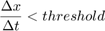
NB: In version v1.3 the method setEpochTrigger will replace the sig.quiescenceWatch. Note that the default threshold for this method is 0, instead of 1.

% Create a signal that represents time
Fs = 2000;
t = 0:1/Fs:0.5;
t = t(1:200);
t = sig.test.sequence(t, 0.1, 'name', 't');

% Create an oscillating signal by adding two sine waves
a = sin(2*pi*400*t); % A sine wave
b = sin(2*pi*375*t); % Another sine wave
x = sig.test.sequence(a + b, 0.1);

duration = (1/Fs)*5; % The quiescence duration in time samples
threshold = 1; % x must change by less than this for the length of duration

% A signal that updates around the max of x, arming our epoch trigger.
% When this updates, its value sets the next epoch duration
newPeriod = at(duration, x > 1.8);
newPeriod.Name = 'duration'; % Rename it for display purposes

% Create our epoch trigger signal
tr = newPeriod.setEpochTrigger(t, x, threshold);

sig.test.timeplot(t, x, newPeriod, tr, 'tWin', 20, 'mode', [2 2 1 1]);

This method is used for enforcing quiescence periods, where the subject must ramain still for a given period of time. Each time the first input, newPeriod updates to a non-zero value, a new quiescence period is enforced.

It can also be used as a sort of timeout, for instance if the subject stops interacting for a given amount of time the session could end automatically, or as a dynamic response window where the trial ends when the movement ceases.

% Reset the 60 second timer when the wheel changes
period = wheel.delta.then(60);
events.expStop = period.setEpochTrigger(t, wheel);

The dimention over which quiescence is enforced doesn't need to be time, it could be another input instead. Likewise, reversing the inputs would impose the oppositeof a quiescence period, where the trigger updates to true when movement reaches threshold within a given amount of time:

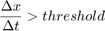
tr = threshold.setEpochTrigger(wheel, t, duration)

merge

The merge method takes any number of inputs and returns the value of the last updated input.

% Here we create four signals that each update in staggered fashion:
x = sig.test.sequence([1 1], 1, 'delay', 1); % Update once per second after a second
a = sig.test.sequence(2, 1, 'name', 'a', 'delay', 2); % Update after 2 seconds
b = sig.test.sequence(3, 1, 'name', 'b', 'delay', 3); % Update after 3 seconds

y = a*x^2 + b*x;

z = merge(x, a, y, b);

sig.test.timeplot(x, a, b, y, z, 'mode', 1, 'tWin', 3);

Unlike most other signals, merge signals update when any of their inputs updates, regardless of whether all their inputs have a value. The order of the inputs is significant: when two signals update simultaneously the value of the input that comes earlier in the list is selected. In the above example 'b' and 'y' update simultaneously (when 'b' updates all of the inputs to 'y' have a value, so 'y' updates). Because 'y' comes before 'b' in the merge list, 'z' takes the value of 'y' rather than 'b'.

If you want the merged signal to update only after all signals have a value, you can use the following:

% Because [a b c] requires all three inputs to have a value, it will only
% start to take values when all are initialized.  Then each time an input
% updates, allUpdated will update to true, this then samples the current
% value of the merge signal for s
allUpdated = map([a b c], true);
s = allUpdated.then(merge(a, b, c));

delay

The delay method produces a signal that updates a given number of seconds after its input.

emitter = sig.test.sequence([-1 -1 0 3 4 4 5], 0.5);

x = emitter.skipRepeats;
y = x.delay(1);

sig.test.timeplot(x, y, 'mode', 1)

As with lag, the number you delay by may be a Signal object:

x = sig.test.sequence(1:5, 1); % a signal that counts to 5
d = x.scan(@plus,0); % each time x updates, delay by sum of values
y = x.delay(d); % update with value of x with ever increasing delay

sig.test.timeplot(x, y, 'mode', 1, 'tWin', 20);

Notes

(1) If a signal already has a value and you derive a new signal from it, the new signal won't automatically compute its value. In the Signals Experiment Framework, the experiment definition function is run once to set up all Signals, before any inputs are posted into the network, so this isn't an issue.

(2) You can get the number of nodes in the network by calling networkInfo on the net id:

networkInfo(a.Node.Net.Id)

Net 0 with 9/4000 active nodes

(3) As you may have noticed from the node graphs, when you evaluate an expression involving a signal, any numbers are made into Signal objects. These are nodes that only ever have one value (known as 'root' nodes). There are often more nodes in a network than you might expect, for example the following line indicates that there are at least 4 nodes in the network:

x = mod(floor(x), 1*2)

These would be x, 2 (a root node), floor(x) and mod(floor(x), 2).

(4) When a function is called on an object, MATLAB checks whether that object's class has a method of the same name (a 'method' is a function that is part of an object's class). If the class has that method associated with it, this method is called instead of the usual function. This is known as 'overloading' and is how we can do things like adding and subtracting Signals. For more info, see the MATLAB documentation here.

(5) This is known as 'syntactic sugar', and a list of MATLAB's operators and the functions they correspond to can be found here.

(6) Specifically, scan performs a left fold. For example for y = x.scan(@plus, 0) where x := {1,5} we get ((((0 + 1) + 2) + 3) + 4) + 5

Summary

Here are the most important things to remember when writing an experiment:

Next section: expDef Inputs.

Bonus plot 1

t = 1.5 : 0.01 : 14.2;
t = sig.test.sequence(t, 0.2);
x = t - 1.6 * cos(24*t);
y = t - 1.6 * sin(25*t);
sig.test.plot(x, y, 'Color', [0 0.4470 0.7410]);

Butterfly curve (transcendental plane curve)

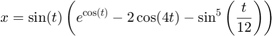
t = sig.test.sequence(0:0.1:12*pi, 0.2);

f = exp(cos(t)) - 2 * cos(4*t) - sin(t/12)^5;

x = sin(t) * f;
y = cos(t) * f;

sig.test.plot(x,y);
xlim = [-5 5]; ylim = [-5 5];

Etc.

Author: Miles Wells

v0.0.4

%#ok<*NASGU,*NOPTS,*ST2NM>

Published with MATLAB® R2019b